How To Make A Cashier Count Chart In Excel - How to create a chart by count of values in Excel? / Once the data is setup we just have to create the chart and put it all together.
regameldiyansah
5 Apr, 2021
How To Make A Cashier Count Chart In Excel - How to create a chart by count of values in Excel? / Once the data is setup we just have to create the chart and put it all together.. Add duration data to the chart. The argument you are entering at the moment is highlighted in bold. This chart can be created in 5 simple steps using a stacked bar chart. What is a funnel chart? Select your data (both columns) and create a pivot table:
On a final note, i would like to do one more thing to our analysis and that is to create a bar chart. Control charts are statistical visual measures to monitor how your process is running over the given period of time. Click smartart, click hierarchy, click organization chart. To generate a chart or graph in excel, you must first provide excel with data to pull from. The argument you are entering at the moment is highlighted in bold.
How to create line graph in excel 2013 - YouTube from i.ytimg.com If i click on cell c22, to make it the active cell, then click on the autosum button in the editing group, the program will enter a formula into the cell. Select your data (both columns) and create a pivot table: And the data looks as below. If you insert a chart in word or powerpoint, a new sheet is opened in excel. As you'll see, creating charts is very easy. A side bar will open in excel for the formatting of the chart. Select data and add series 5. In the menu in the subgroup of label options you need to uncheck the value and put the checkmark on percentage.
Putting the chart & dashboard together.
To create a line chart, execute the following steps. Once again right click on the chart and select the item format data labels: Select a black cell, and press ctrl + v keys to paste the selected column. Would you like to be able to show completed and not completed a. Since the chart is interactive, it's best if the names in the legend are also updated when the user changes the chart. Now select the pivot table data and create your pie chart as. You can create a chart in excel, word, and powerpoint. Enter the data you want to use to create a graph or chart. The select data source window will open. Select your data (both columns) and create a pivot table: Position your charts in a range, one chart per cell select a range of cells and resize them so that each cell can accommodate one chart. The argument you are entering at the moment is highlighted in bold. Once the data is setup we just have to create the chart and put it all together.
The marks column will get sorted from smallest to largest. As you'll see, creating charts is very easy. Control charts are statistical visual measures to monitor how your process is running over the given period of time. Microsoft excel will display the function's arguments as soon as you start typing; You can create a chart in excel, word, and powerpoint.
How to make a bar graph in Excel (Scientific data) - YouTube from i.ytimg.com Enter data into a worksheet. Select the fruit column you will create a chart based on, and press ctrl + c keys to copy. Select data and add series 5. And the data looks as below. Introduction to control charts in excel. The shape (which is a rectangle) at the top of the chart is the head of the organization. The argument you are entering at the moment is highlighted in bold. Select chart and click on select data button.
Select the fruit column you will create a chart based on, and press ctrl + c keys to copy.
Add duration data to the chart. Control charts are statistical visual measures to monitor how your process is running over the given period of time. On a final note, i would like to do one more thing to our analysis and that is to create a bar chart. You can use the countifs function in excel to count cells in a single range with a single condition as well as in multiple ranges with multiple conditions. Across the top row, (start with box a1), enter headings for the type of information you will enter into your run chart: Enter data into a worksheet. The first chart uses the correct names but the second chart the data that has an incorrect country name caneda. Would you like to be able to show completed and not completed a. And the data looks as below. To create a line chart, execute the following steps. Then click on add button and select e3:e6 in series values and keep series name blank. Position your charts in a range, one chart per cell select a range of cells and resize them so that each cell can accommodate one chart. You can create a chart in excel, word, and powerpoint.
Now select the pivot table data and create your pie chart as. A simple chart in excel can say more than a sheet full of numbers. Microsoft excel will display the function's arguments as soon as you start typing; Click smartart, click hierarchy, click organization chart. In this section, we'll show you how to chart data in excel 2016.
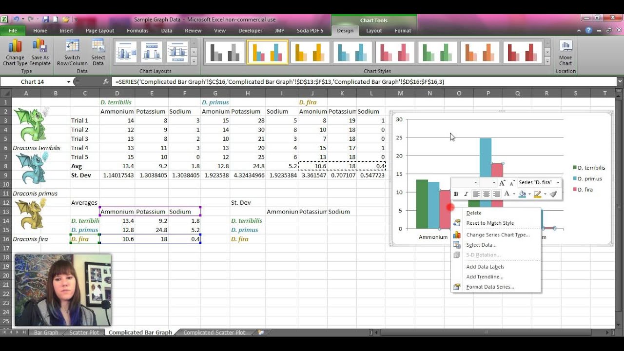
How to Build a More Complicated Bar Graph in Excel - YouTube from i.ytimg.com A side bar will open in excel for the formatting of the chart. This has been a guide to grouped bar chart. Here, reduce the series overlap to 0. Select the fruit column you will create a chart based on, and press ctrl + c keys to copy. However, the chart data is entered and saved in an excel worksheet. You can create a chart in excel, word, and powerpoint. To do so, all you have to do is to highlight the model and frequency categories and click the insert tab to create the bar chart: Select the data range and choose clustered column chart from the insert chart menu.
I can also use the editing group, on the home tab, to add up, count and find the averages of selections of number data.
Once again right click on the chart and select the item format data labels: I can also use the editing group, on the home tab, to add up, count and find the averages of selections of number data. Click that rectangle (you may need to move or hide the text pane) and type the name of that person. Whether it is running as expected or there are some issues with it. The argument you are entering at the moment is highlighted in bold. Select your data (both columns) and create a pivot table: Open excel and select new workbook. Here we discuss how to create a grouped bar chart in excel along with a practical example and a downloadable template. Once the data is setup we just have to create the chart and put it all together. Click on the series option. Would you like to be able to show completed and not completed a. To create a line chart, execute the following steps. Select the fruit column you will create a chart based on, and press ctrl + c keys to copy.